![]()
![]()
![]()
![]()
|
|
|
|
|
The fitting methods available optimize the agreement between the measurements and the model curve. Effectively, they minimize the difference between them, whereby the difference is described by the Chi Squares criterion (cost function):
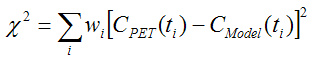
This expression implies that the squared residuals (measured value minus estimated model value) are multiplied by weights. To satisfy the requirements of least squares fitting, the weights wj should be related to the standard error sj of the measurements by
![]()
In this case, and provided that the distributions of the measurement error are normal, the estimate obtained is the maximum likelihood estimate. Under the same premise it is also possible to obtain standard errors of the model parameters as the square root of the diagonal elements in the covariance matrix.
In PKIN, several different weight definitions are supported. They can be specified using the selection besides Weighting.
The selection shows the assumed error distribution (Gaussian, Poisson or Uniform). The distribution type is not relevant for fitting, only for Monte Carlo simulations where noisy curves must be generated.
For fitting, only the standard deviations si are needed. These can be specified as follows: Activate the distribution button (eg. Gaussian). In the appearing dialog select the list Formula for calculating standard dev. It shows the entries:
L*mean(y) |
Use the average of all measurements multiplied by the factor L as an estimate of s. This setting with L=0.05 (5%) is the default. |
L*max(y) |
Use the maximal measurement value multiplied by the factor L as an estimate of s. |
L*y |
Use the measurements multiplied by the factor L as an estimate of si . |
L*sqrt(y) |
Use the square root of the measurements multiplied by the factor L as an estimate of si (Poisson distribution; is adequate for counting radioactivity, but not necessarily for reconstructed activity concentrations). |
unity 1.0 |
Sets s = 1.0. |
L*measured |
Uses a scaled vector of standard errors which has been imported. Most likely, L should be set to 1.0. |
[CONSTANT] |
This annotation indicates that one single s is used for all measurements over time. As a consequence, unweighted fitting is performed. All measurements have the same impact on the fit result. |
[VARIABLE] |
Indicates that an individual si is used for weighing the residual at each time point. As a consequence, weighted fitting is performed. Noisier measurements (larger si) have less impact on the outcome. |
Each time the configuration is changed, the standard error is calculated and plotted as an error bar around the measurements. This feedback should give the user some feeling for the adequacy of the specified distribution.
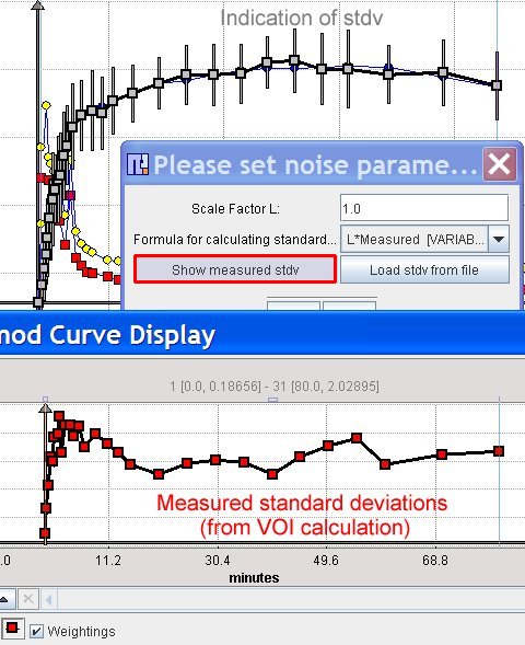
Note that the dialog box allows to load externally measured standard errors. Activate Load stdv from file and select a text file of the form
t[seconds] |
|
v[1/1] |
0 |
|
0.10300076 |
20 |
|
0.01717448 |
40 |
|
0.01195735 |
60 |
|
0.01010257 |
etc |
|
... |
The header line is required. The first column represents the frame times (the values are not interpreted), and the second column the standard deviations in appropriate units. The number of entries must be equal the number of acquisitions, and the columns separated by spaces or tabs. For example, the file can be prepared in Excel and then saving as a text file with tab delineation.
An approximation of measured standard errors is automatically available, if the TAC data have been sent directly from PVIEW to PKIN. They represent the standard deviation of the activity within the VOI at each time point.
In the Standard mode the si resulting from the Weighting settings can be visualized as gray error bars by the Show noise check.