![]()
![]()
![]()
![]()
|
|
|
|
|
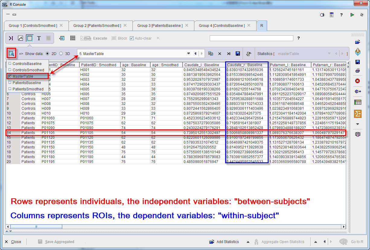
The data structure to be used in the linear models statistical analysis can best be visualised by a master table where columns represent regions and rows represent individuals. To build up the master table, aggregated files are required. It is essential that consistent group and condition names are correctly encoded for each aggregated file. Detail information about the aggregation procedure is available above.
Statistically, individuals (rows) are independent from each other while regions (columns) are not, which is an important distinction for the analysis structure. Each classification axis can have further subdivisions. E.g., individuals could be split into experimental groups, while the same regions might be present in the left and the right brain hemisphere. We would then have the experimental group classification as a “between-subject” variable, and regions and hemispheres as nested “within-subject” variables.
In-vivo imaging studies will often repeat scans in the same individuals. One could then analyse the difference between baseline and follow-up as the dependent variable of interest. Alternatively, measurement instance (baseline and repeat, optionally also further repeat measurements) could be represented as a within-subject variable (analysing the same set of regions at all measurement times). Note, that repeat measurements would not represent another group of individuals, thus they are to be added as columns, not as rows.
The example below illustrates how to build the master table. To this purpose, four aggregates were created and transferred to the R console. Two groups, Control and Patient were analyzed in two conditions: Baseline and Smoothed. Please note that an aggregate was prepared beforehand for each group and condition.
Use the master table  icon from the lateral taskbar to start the interface for preparing the data for population statistics.
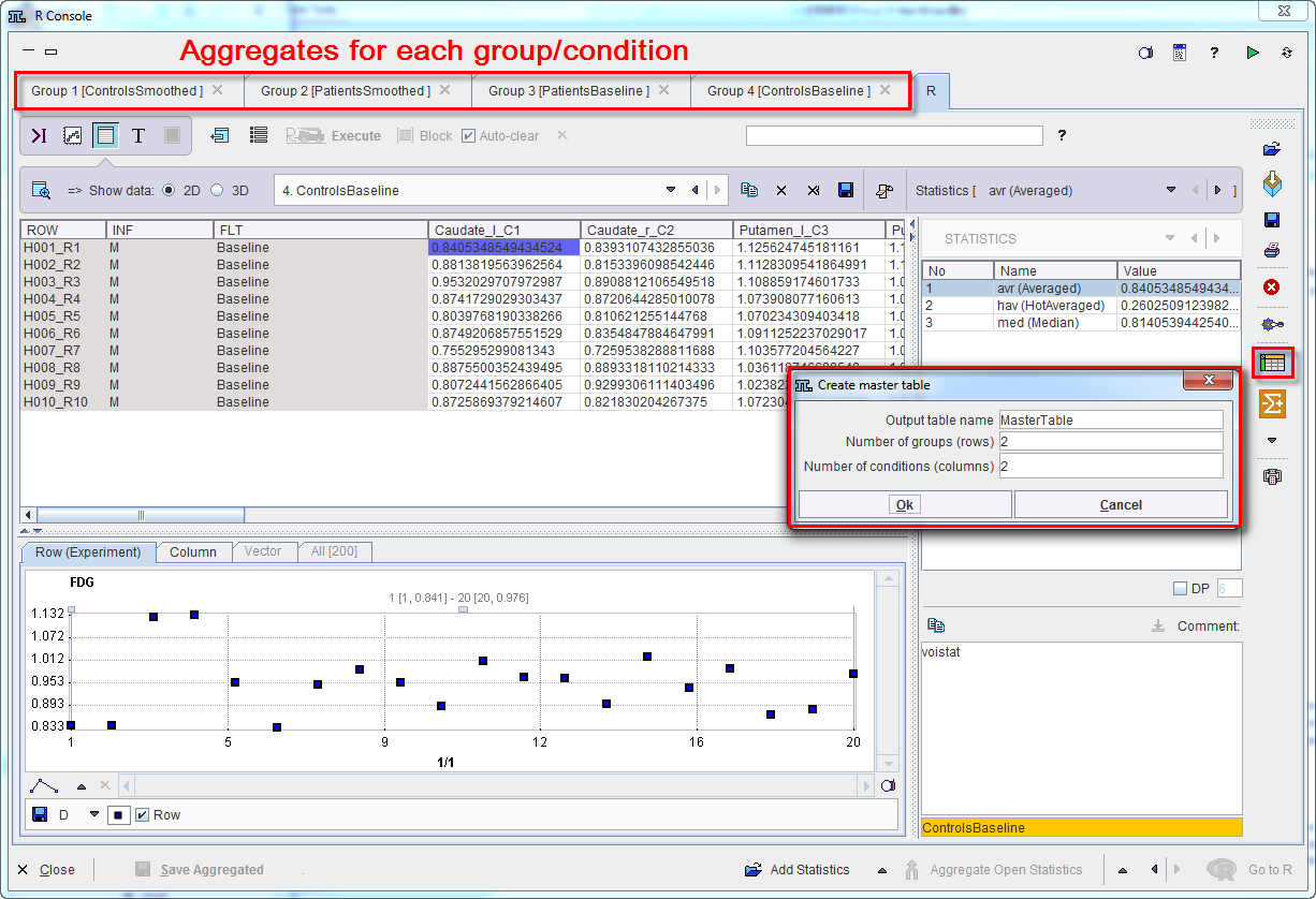
A dialog window opens allowing the definition of the number of rows and columns for the master table. The rows and columns correspond to the groups and conditions, respectively. The name of the master table can be edited in the Output table name field. To continue activate the OK button.
The Master table creator interface appears:
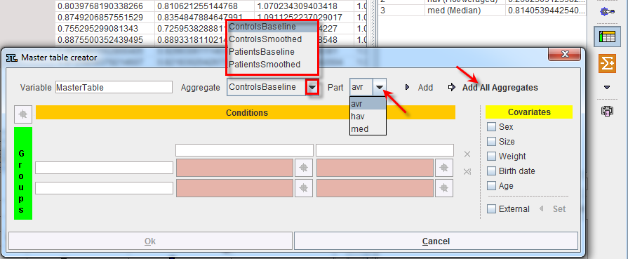
To fill in the master table select the Aggregate file to start with and the statistics Part to be analyzed. To transfer the avr part of all aggregates to the master table activate Add all Aggregates. The procedure uses the group and condition names encoded during aggregation for the arrangement of the aggregates in the table. This step will not work properly if the encoding was not consistent.
The result of the example is shown below:
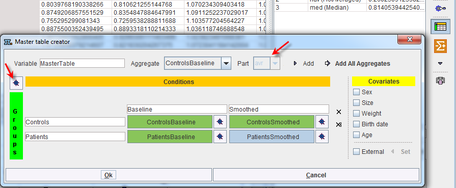
The master table has a structure consisting in blocks, each block corresponding to a group and condition. To preview the content of the master table activate the View value icons  as indicated below:
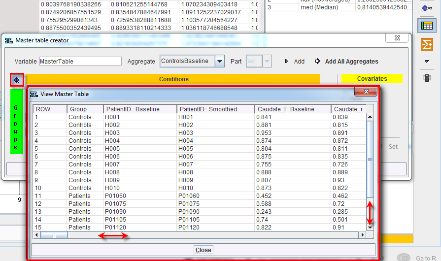
Use the bar sliders to navigate through the master table content preview. Similarly, the content of each element of the master table can be visualized.
Individuals may also be characterised by additional variables. These can be demographic variables, such as sex and age, or experimental variables, such as functional performance scores. Researchers will often be interested in the effect of these variables on regional values.
The covariates can be easily included in the master table by enabling the corresponding checkboxes in the Covariates section:
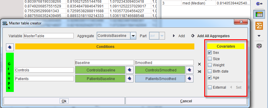
Please note that the covariates have to be available in the aggregates for each condition and group. Alternatively, they can be loaded as External files during the loading procedure of the aggregate. To transfer the external information to the master table the External checkbox has to be enabled and the Set button activated. Statistically they are treated as covariates, and they are added as extra columns to the master table. Logically, these additional columns represent independent variables, while the columns of regional values are dependent variables.
Finally, to instantiate the master table, activate the Ok button. A new Variable MasterTable is added to the workspace. It can be visualized in the Table layout as shown below: