![]()
![]()
![]()
![]()
|
|
|
|
|
Note that if Linearity corr is enabled there are two choices:
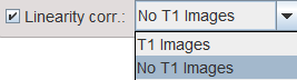
During the TAC calculation, a corresponding dialog window will open .
T1 Images
With the first T1 images choice an image selection window opens. The user has to select the T1 scan which corresponds to the perfusion data set being analyzed, eg. T1 STRESS. PCARDM will load the images, interpolate them to the geometry of the perfusion scan and then show them in a window as illustrated below. A mask of the myocardium and the LV derived from the segmentation are shown in the overlay. It is the task of the user to shift the mask by dragging the handle such that it fits to the anatomy as illustrated below.

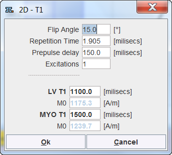
The program reads sequence parameters from the T1 scan file and uses them for fitting an average T1 time for the left ventricle (LV T1) and the myocardium (MYO T1) from the recovery of the magnetization. These values are shown in the fit results section. LV T1 will be used for correcting the LV TAC, and MYO T1 for correcting all segmental TACs.
No T1 Images
If no T1 images are available the relevant information can be manually entered into a dialog window.
Correction Procedure
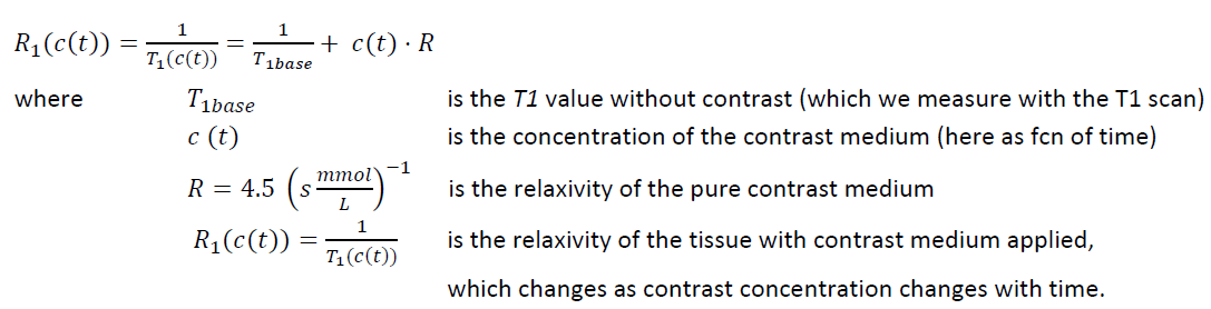
In principle the relaxivity R1 is first calculated [4]:
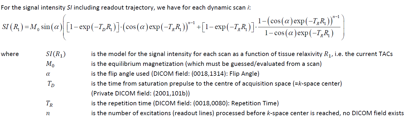
R1 is then applied for the conversion from MR signal to contrast agent concentration by [4]:
After a segmentation scheme has been applied and the time-contrast curves calculated, they are shown in the lower left on the MODELING page.
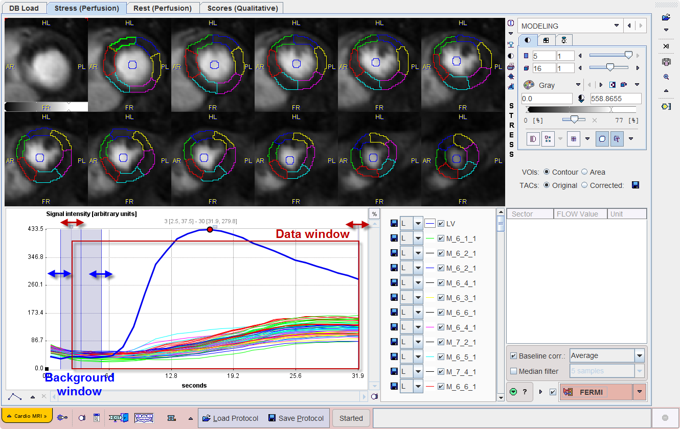
The LV curve represents the concentration of contrast agent in the center of the LV cavity. It should rise earlier than the segmental curves as the contrast arrives first in the ventricle, before being transported to the myocardium via the coronary artery system.
Baseline Correction
The concentration of contrast agent should be zero before arrival of the contrast bolus. The MR signal, however is not zero. Assuming that the relation between contrast concentration and MR signal is similar in blood and myocardium, the baseline signal of each curve can be subtracted to arrive at an approximate contrast curve.
Baseline correction can be enabled with the Baseline corr box. Correspondingly, a blue shaded area is shown in the curve area. It should be adjusted such that it covers a sufficient window before the signal rise. There are 4 choices for the curve correction:
With Average (recommended), the signal average in the background window will be calculated for each curve, and then subtracted. The Minimum setting works similarly with the minimal value in the baseline window.
The Norm (Ref) and Norm (TACs) choices normalize the curves in a different way. They are aimed at correcting regional coil sensitivity differences [5]. With Norm(Ref) a calibration factor is calculated from the relative baselines of the TAC and the LV. With Norm (TACs) the calibration factor is calculated from the TAC baseline and the average of all TAC baselines.
Signal Filter
In order to filter noisy signals a Median filter can be enabled. It allows filter widths of 5, 7 and 9 samples which are applied along the time. An advantage of using the median is that it does not affect the upslope shape.
Data Cropping
A data window can be placed to crop the signal in the time domain as illustrated above. Default is to use the whole signal. Please drag the handles to reduce the window, for instance to remove most of the baseline signal, and to cut a tail affected by recirculation.
Starting the quantification
The curves which will be used for quantification can be visualized by enabling the Corrected radio button in the TACs area. For the quantification it is important that the LV curve starts from a value close to zero and the upslope part is not truncated.

The red action button in the lower right starts the quantification. It has three settings which correspond to the quantification model which is applied to the curves. Recommended is the FERMI model.

Note the check box next to the action button. If it is enabled, the program module applied for the quantification will open with loaded data, and the user can perform the curve modeling interactively. The advantage is that the outcome can be easily inspected, and any failures most probably fixed as described in the next section.
Otherwise, the quantification is performed in the background and the resulting perfusion values returned for the results display. Quantification failures in the segments are indicated by returning NaN values.