Residence Times

The Residence Times model performs pre-processing steps for the calculation of the absorbed dose from diagnostic or therapeutic radiopharmaceuticals. Given the time-course of the activity in a volume of tissue, it calculates the Residence Time, which should better be called the Normalized Cumulated Activity [1] to avoid confusion of its meaning. It represents the total number of disintegrations which have occurred during an integration time per unit administered activity. Ideally, integration is performed from the time of administration to infinity. However, as it is widely used in literature, the notion Residence Time will be used in the remainder of this section.

The organ residence times resulting from the Residence Times model can serve as input to a program such as OLINDA [2] for the actual calculation of the absorbed organ doses.

Operational Equations

Given an activity A₀ applied to a subject, and a measured (not decay corrected) activity A(t) in an organ, the residence time t is calculated by

Note that the unit of t is usually given as [Bq×hr/Bq]. The measured part of the organ activity can easily be numerically integrated by the trapezoidal rule. For the unknown remainder of A(t) till infinity it is a conservative assumption to apply the radioactive decay of the isotope. This exponential area can easily be calculated and added to the trapezoidal area. Alternatively, if the measured activity curve has a dominant washout shape, a sum of exponentials can be fitted to the to the measured data and the entire integral algebraically calculated.

The Residence Times model in PKIN supports both the trapezoidal integration approach as well as the use of fitted exponentials. It furthermore supports some paracticalities such as

conversion of an average activity concentration in [kBq/cc] to activity in [Bq] by multiplication with the VOI volume;
reversion of decay correction;

Model Input Parameters

The Residence Times model has 4 input parameters which need to be specified interactively by the user. These settings can easily be propagated from one region to all others with the Model & Par button.

Decay corrected	Check this box if the loaded curves have been decay corrected as is usually the case for PET imaging studies. The Halflife of the radioisotope will be used to undo the decay correction.
Activity concentration	Check this box if the loaded curves represent activity concentration rather than the total activity in a region. The volume of the region will be multiplied with the signal to calculate activity in [Bq].
Isotope tail	Check this box to use the radioactive decay shape for the integration from the end of the last frame to infinity. This option is only relevant if exponentials are fitted to the measurement. For the Rectangle and Trapezoid methods it will always be added.
Integration	The integration method can be selected in the option list: Rectangle, Trapezoid, 1 Exponential, 2 Exponentials, 3 Exponentials. The Rectangle method is the natural selection for PET values which represent the time average during the frame duration. If there are gaps between the PET frames, the uncovered area is approximated by the trapezoidal rule. The Trapezoid method uses trapezoidal areas between the frame mid-times. With an Exponential selection, the specified number of decaying exponentials is fitted to the measurements, and used for analytical integration. Note that samples marked as invalid are neglected in the fit.

Editing of Constituents

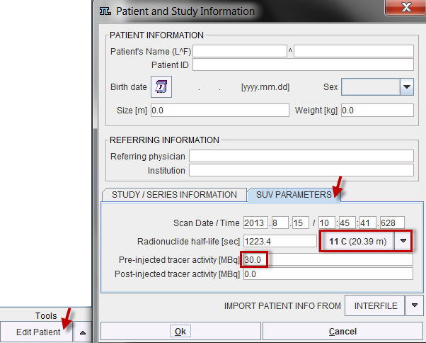
Depending on the import of the activity curves, isotope and activity information may or may not be available. They can be edited in the Patient and Study Information window as illustrated below. Activate Edit Patient in the Tools list, select SUV PARAMETERS, and enter Radionuclide half-life and Pre-injected tracer activity. Note that the activity needs to be calibrated to time 0 of the activity curve.

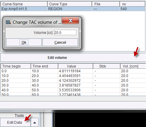
The region volume is available if the TAC was generated in PMOD's View tool and transferred to PKIN. Otherwise the volume has to be entered as illustrated below. Activate Edit Data in the Tools list, select a region in the upper list, then activate Edit volume from the curve tools and enter the Volume number.

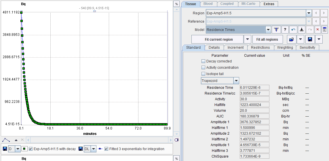
Model Output Parameters

As soon as the Fit Region button is activated, the fits and calculations are performed, resulting in a list of parameters:

Residence Time [Bq×hr/Bq]	Total number of disintegrations in region from time 0 until infinity. The main result and equal to AUC/Activity.
Residence Time/cc [Bq/cc×hr/Bq]	Total number of disintegrations per unit volume in the region. Equal to AUC/(Activity×Volume). If the organ has deliberately been outlined within the organ to reduce the partial-volume problem, Residence Time/cc may be multiplied with the actual organ size to approximate the activity taken up. The residence time for standard phantom organs can be easily be calculated by multiplying the tabulated organ mass with Residence Time/cc and dividing by the organ density (usually 1g/ccm).
Activity [MBq]	Administered activity. Shown for verification only.
Halflife [sec]	Isotope halflife. Shown for verification only.
Volume [ccm]	Region volume. Shown for verification only.
AUC [Bq×hr]	Integral of the activity curve from time 0 till infinity.
Amplitude 1, 2, 3 [Bq] Halftime 1, 2, 3 [min]	Amplitudes and halftimes of the fitted exponentials. In the case of 1 exponential a linear regression is applied, whereas iterative fitting is used with 2 or 3 exponentials.

Reference

1. Stabin MG: Fundamentals of Nuclear Medicine Dosimetry. Springer; 2008. DOI

2. Stabin MG, Sparks RB, Crowe E: OLINDA/EXM: the second-generation personal computer software for internal dose assessment in nuclear medicine. J Nucl Med 2005, 46(6):1023-1027.